Pixel Recurrent Neural Networks
Paper Summary: Pixel Recurrent Neural Networks
1. Intro
생성 모델은 비지도학습(unsupervised learning)으로, 주어진 데이터의 분포(probabilistic density)를 학습하여 그 분포에 포함되는 새로운 데이터를 샘플링하는 방법이다. 특히 이 방법은 이미지 데이터의 inpainting, deblurring과 같은 복원 과정에 사용될 수 있다. 하지만 이미지 데이터의 분포는 굉장히 복잡하여, 이 분포를 잘 표현하면서 tractable하고 scalable한 모델을 만드는 것은 굉장히 어렵다.
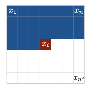
Tractable이라 함은 학습한 데이터의 분포를 직접적으로 알 수 있음을 이야기하는데, 이에 대한 한 가지 방법으로 autoregressive 모델을 사용할 수 있다. 이는 예측할 joint distribution을 factorizing하여 각 conditional distribution을 예측하게 하는 것이다.
식 (1)에서
또한, 각 픽셀은 Red, Green, Blue의 세 개의 채널 값을 가지고 있는데 이 값들 또한 factorizing하여 아래와 같이 표현할 수 있다.
이러한 conditional distribution을 예측할 때, 멀리 있는 픽셀들 사이의 long-range correlation과 같은 복잡한 분포를 표현할 수 있어야 하므로 적절한 architecture가 필요하다. 본 논문에서는 recurrent neural networks (RNN)을 사용하였는데, 특히 two-dimensional long short-term memory (LSTM) layer를 사용하여 모델을 구현하였다. 추가적으로, 깊게 LSTM layer를 쌓기 위해 residual connection을 사용하였다.
또한, 연속적인 분포를 사용한 기존 연구들과 다르게 각 conditional distribution을
2. Main Contributions
본 논문에서는 네 가지의 모델을 소개하고 있다.
- PixelRNN with Row LSTM layer
- PixelRNN with Diagonal BiLSTM layer
- PixelCNN
- Multi-scale PixelRNN
한 가지씩 살펴보고, 각 모델에 대한 결과를 알아보자.
PixelRNN
a. LSTM
LSTM은 기본적으로 input-to-state와 state-to-state 파트로 이루어져 있다. 기존의 two-dimensional LSTM은 식 (3)과 같이 hidden-state
b. Row LSTM
Row LSTM은 위의 단점을 보완하기 위한 한 가지 방법으로, row 단위로
c. Diagonal BiLSTM
주어진 모든 이전 픽셀 정보를 활용하여 다음 픽셀을 예측하기 위해 제안된 방법이 Diagonal BiLSTM이다. 이를 수행하기 위해서 Fig 3.과 같이 기존 이미지의 각 row를 윗 row에 비해서 한 칸씩 오른쪽으로 skewing하는 pre-processing을 한다. 이후 식 (5)와 같이 column-wise
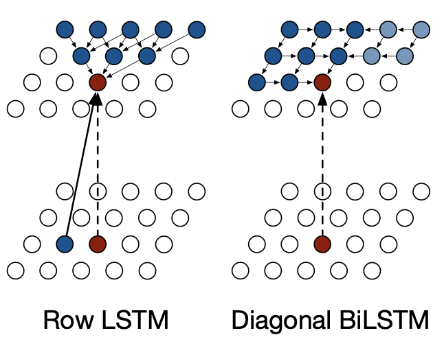
Fig 2. Illustration of the Row LSTM and the Diagonal BiLSTM 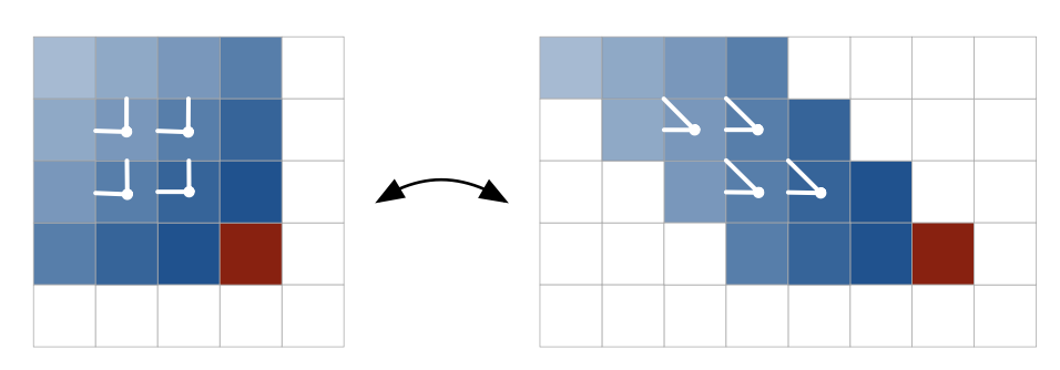
Fig 3. Skewing operation of the input map for the Diagonal BiLSTM PixelCNN
RNN에 비해서 computational cost를 낮추기 위한 방법으로 masked CNN을 사용하였다. Fig 4.와 같이 아직 예측하지 않은 pixel을 masking한 kernel을 이용하여 convolution을 수행하였다. 이렇게 하면 recurrent한 계산을 하지 않고 모든 픽셀에 대한 값을 한 번에 계산할 수 있어 속도가 빠르지만 bounded receptive field로 인하여 long-range correlation은 고려하지 못한다(blind spot).
)](https://github.com/WonhoZhung/starter-academic/blob/master/images/post4/Untitled%203.png?raw=true)
Fig 4. Illustration of the PixelCNN (Source: http://slazebni.cs.illinois.edu/spring17/lec13_advanced.pdf) Multi-scale PixelRNN
먼저 기존 이미지의 subsampled 이미지를 PixelRNN으로 생성한 후, 이로부터 deconvolution layer를 통해 다시 원래 크기의 이미지를 생성하는 방식이다.
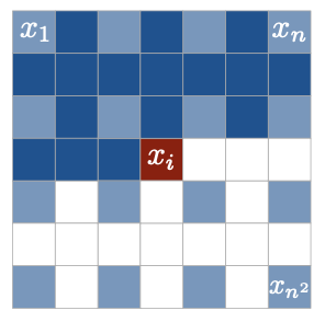
Fig 5. Illustration of multi-scale case
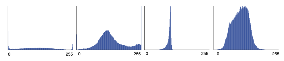
이제 결과를 살펴보자. 먼저 눈여겨볼 부분은 역시 각 픽셀 RGB 채널의 tractable한 probability distribution이다. Fig 6.과 같이, 모델에 불연속적인 분포를 사용하였음에도 well-behaving하는 확률 분포를 보여주었다.
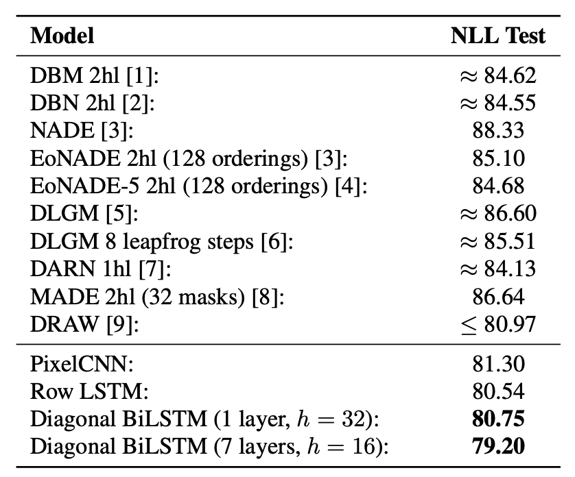
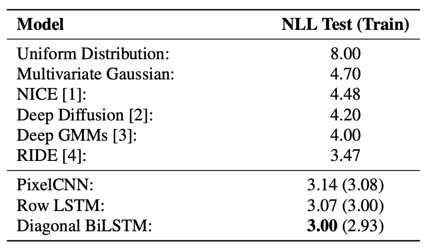
본 논문에서는 MNIST, CIFAR-10 데이터셋에 대해 모델 성능을 평가하였다. 기존의 모델들의 성능보다 state-of-the-art를 보여주었다. 특히, Diagonal BiLSTM의 넓은 receptive field 덕분에 이 경우 가장 좋은 성능을 보여주었다.
3. Opinion
본 논문은 autoregressive model의 정석으로, sequential하게 픽셀의 conditional distribution을 구하는 방식으로 이미지를 생성하는 방법론을 소개하였다. 특히, Diagonal BiLSTM을 사용하여 PixelRNN에서 parallelization을 가능하게 하는 동시에 이미지 크기에 상관없이 모든 context를 포함하게 한 아이디어가 인상적이었다. 아래는 논문을 읽으며 생각한 discussion point들이다.
- How can the autoregressive model control the randomness of the sampling?
- What if we train/generate the model in other sequential paths of image pixel rather than from top-left to bottom-right?
- Can we use attention to interpret the long-range correlations between pixels?
Wonho Zhung
Ph.D. Candidate, KAIST
My research interests include applying deep learning to solve problems in chemistry and biology.