NVAE: A Deep Hierarchical Variational Autoencoder

Paper Summary: NVAE: A Deep Hierarchical Variational Autoencoder

1. Intro

“In this paper, we aim to make VAEs great again by architecture design.”

Variational auto-encoder (VAE)는 Fig 1.와 같이 주어진 데이터를 latent vector space로 압축했다가 다시 reconstruct하는 auto-encoder의 구조를 가지고 있지만, latent vector $z$가 deterministic하게 결정되는 것이 아니라 variational inferencing을 통해 정해진 distribution $q_ \phi (z|x)$으로 부터 sampling 된다는 특징을 가진다. VAE의 objective function은 아래의 식 (1)과 같으며, 전자의 reconstruction loss와 후자의 KL regularization loss로 이루어져 있다.

$$\tag{1} \mathcal{L}_ {VAE}(\theta,\phi)=-\mathbb{E}_ {z\sim q_ \phi (z|x)}[logp_ \theta (x|z)]+KL(q_ \phi (z|x)\Vert p_ \theta (z))$$

VAE는 latent vector를 이용한 interpolation이나 conditioning이 가능하다는 단점이 있지만, Fig 2.와 같이 GAN에 비해서 blurry한 이미지를 생성한다는 단점이 있다. 이는 posterior의 분포를 Gaussian으로 가정하면서 동시에 L2 loss를 감소하는 방향으로 학습을 진행하여 발생하는 문제이다.

기존의 연구들에서는 VAE의 이러한 단점을 극복하기 위하여 아래와 같은 statistical challenges에 집중하였다.

• Reducing the gap between approximate and true posterior distributions
• Formulating tighter bounds
• Reducing the gradient noise
• Extending VAEs to discrete variables
• Tackling Posterior collapse or prior hole

본 연구에서는 이러한 접근법과 다르게, model architecture만을 가지고 VAE의 성능을 개선하는데에 기여하였다. Hierarchical 구조로 VAE를 쌓아 posterior 분포의 expressive power를 향상시켰으며, unbounded KL divergence로 인해 deep VAE의 학습이 불안정한 문제를 기존의 여러 아이디어를 결합하여 해결하였다. 또한, VAE의 메모리 사용을 줄이기 위하여 테크니컬한 몇 가지 기믹들을 사용하였다.

2. Main Contributions

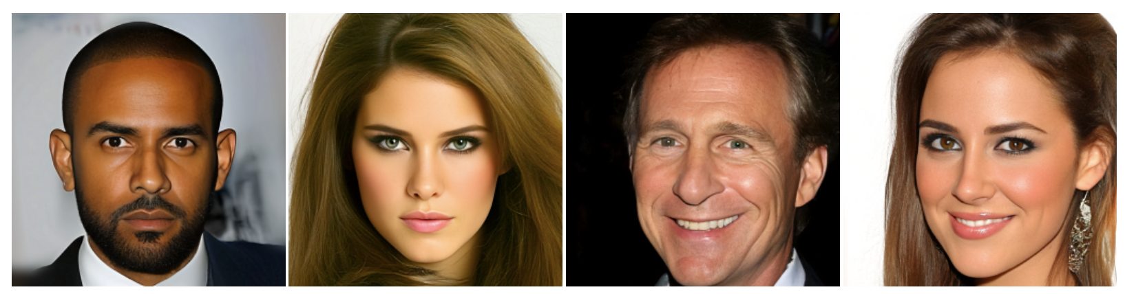
본 논문에서는 Nouveau VAE (NVAE)라는 deep hierarchical VAE 구조를 제안하였으며, 기존 non-autoregressive likelihood-based 생성 모델 중에서 SOTA를 갱신하였다. 먼저 Fig 3.의 NVAE로부터 생성된 이미지를 몇 개 보자. 위의 Fig 2.에서 VAE에 의해 생성된 이미지와는 차원이 다른 선명함을 선명함을 보여준다!

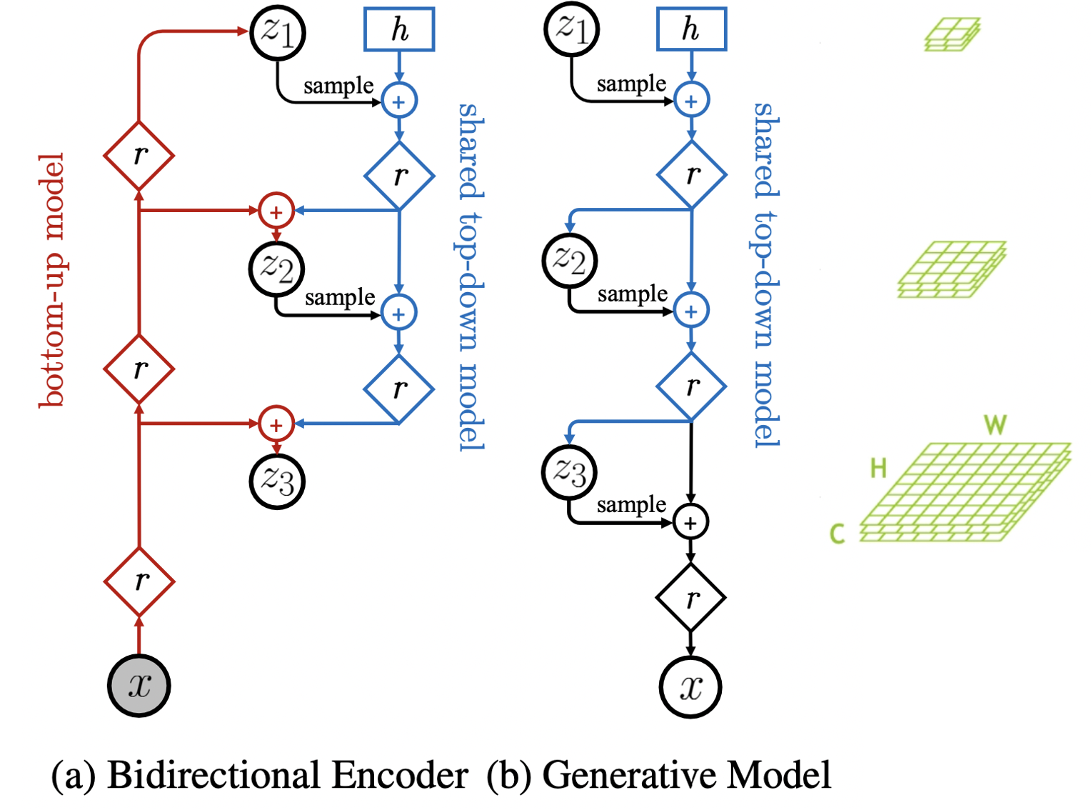
그럼 본격적으로 NVAE의 자세한 architecture를 살펴보자. 전체적인 구조는 Fig 4.와 같이 bidirectional encoder와 decoder(generative model)로 이루어져있다. Latent space가 $L$개의 group으로 이루어져있을 때, prior $p(z)$와 posterior $q(z|x)$는 식 (3)과 같이 표현된다. 설명의 편의를 위해 $z_1$을 위쪽, $z_L$을 아래쪽 group이라고 명명하겠다.

$$\tag{2} z={z_1,…,z_L}$$

$$\tag{3}p(z)=\prod_l p(z_l|z_{<l}),q(z|x)=\prod_l p(z_l|z_{<l},x)$$

Fig 4. (a)의 bidirectional encoder 구조는 input으로부터 최상층의 latent vector로 encoding하는 bottom-up model과 윗 계층의 latent vector로 부터 아래층의 latent vector를 얻는 top-down model이 공존한다. 눈여겨볼 점은 기존 VAE의 encoder와 다르게 encoder에도 sampling이 들어간다는 것이다. 또한, 위에서 아래로 내려갈수록 latent vector의 크기가 점점 커져 압축된 정보로부터 원래의 정보를 복원하게 된다. Fig 4. (b)의 decoder 구조는 encoder의 top-down model을 공유하여, 순차적으로 latent space에서 sampling을 하여 이미지를 생성한다.

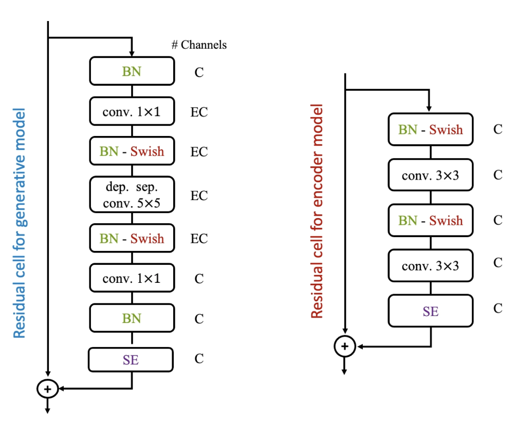
각 계층을 넘어갈 때 Fig 5.와 같은 residual cell을 이용한다. 특히 본 논문에서는 batch normalization을 convolution과 함께 활용하였는데, sampling 과정에서 batch nomalization의 momentum parameter를 조정하여 생성된 이미지의 질과 다양성을 향상시킬 수 있었다. 또한, $1\times 1$ convolution 사이에 depthwise separable convolution을 하여 효과적으로 parameter 수를 줄일 수 있었다.

이러한 deep hierarchical architecture에서 unbounded KL divergence가 안정적으로 optimize 되기 위해서 본 논문에서는 두 가지 방법을 사용하였다.

1. Residual normal distribution

   첫 번째 방법은 residual distribution으로, $q(z|x)$의 분포를 $p(z)$에 상대적으로 나타내는 방법이다. $i$번째 변수의 prior distribution을 식 (4)와 같다고 했을 때, approximate posterior의 분포를 $\Delta\mu_i$와 $\Delta\sigma_i$를 통해 식 (5)와 같이 나타낼 수 있다. 이와 같은 residual distribution에 대해 $\mathcal{L}_{VAE}$의 KL term을 정리하면 식 (6)과 같이 되는데, decoder로부터 학습된 $\sigma$가 아래로 bounded 되어 있으면 encoder에 의해 정해지는 relative parameter로 KL term이 결정됨을 알 수 있다. 이러한 방법을 사용하여 KL term을 보다 간단히 minimize 할 수 있다.

   $$\tag{4} p(z^i):=\mathcal{N}(\mu_i,\sigma_i)$$

   $$\tag{5} q(z^i|x):=\mathcal{N}(\mu_i+\Delta\mu_i,\sigma_i\cdot\Delta\sigma_i)$$

   $$\tag{6} KL(q(z|x)\Vert p(z))=\frac{1}{2}\left(\frac{\Delta\mu^2}{\sigma^2}+\Delta\sigma^2-log\Delta\sigma^2-1\right)$$

2. Spectral regularization

   두 번째 방법은 KL을 보다 직접적으로 bound 시켜주기 위하여 보다 수학적인 방법을 사용한다. Input의 변화가 encoder output에 극적인 변화를 가져오는 것을 방지하기 위하여 Lipschitz constant를 함께 최소화해주는 방법을 사용한다. 이러한 regularization은 encoder를 일정 범위 안으로 bound 시켜 안정적으로 minimize 될 수 있도록 한다. 이를 위해 intractable한 Lipschitz constant 대신 spectral regularization을 사용하며, 각 layer의 singular value 중 최댓값 $s^{(i)}$을 loss에 추가해준다. $\lambda$는 smoothness를 조절해주는 hyper-parameter이다.

   $$\tag{7}\mathcal{L}_{SR}=\lambda\sum_i s^{(i)}$$

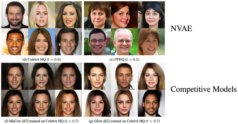
이제 본격적으로 주요 결과들을 살펴보자. Fig 6. (g)에서 GLOW는 autoregressive를 사용하지 않은 flow model인데, 얼굴의 좌우 대칭이나 배경의 long-range correlation이 잘 반영되지 않은 모습이다. 반면 (d, e)의 NVAE가 생성한 이미지는 이러한 correlation이 잘 반영된 것을 학인할 수 있었다. 또한, autoregressive를 사용한 MaCow가 생성한 이미지 (f)에 비해 더 diverse한 이미지를 생성하였다.

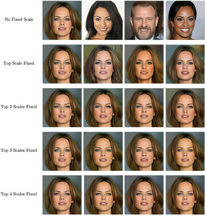
특히 인상적이었던 결과는 Fig 7.인데, $8\times 8$부터 $128\times 128$까지의 5개의 latent group을 각각 고정했을 때 생성되는 이미지로부터 어느 계층에서 global structure가 결정이 되는지를 확인한 실험이다. 최상층의 latent vector를 고정하였을 때 전체적인 이미지는 결정된 채로 피부색이나 입술 모양과 같은 세부적인 특징들만 바뀐 반면, 최상층의 latent vector가 다르게 sampling 되면 완전히 다른 이미지가 생성되는 것을 볼 수 있다. 따라서 첫 번째 hierarchy에 의해 long-range global structure가 결정됨을 알 수 있었다.

3. Opinion

본 논문은 정교한 hierarchical architecture 디자인만으로 VAE로부터 선명한 고화질의 이미지가 생성될 수 있음을 보여주었다. 아래는 논문을 읽으면서 생각이 든 discussion point들이다.

• What is the correlation between the number of hierarchical groups and the model performance?
• How does the latent vector interpolation of each hierarchical group affect the generated image?
• Can this network architecture be applied to tasks other than image generation?
  • such as graph generation, 3D point cloud generation, etc.
• What if the model utilizes the discriminator (like GAN) at the end of the decoder?

$$***$$